Factorial ANOVA

17. Factorial ANOVA#

Over the course of the last few chapters you can probably detect a general trend. We started out looking at tools that you can use to compare two groups to one another, most notably the \(t\)-test. Then, we introduced analysis of variance (ANOVA) as a method for comparing more than two groups. The chapter on regression covered a somewhat different topic, but in doing so it introduced a powerful new idea: building statistical models that have multiple predictor variables used to explain a single outcome variable. For instance, a regression model could be used to predict the number of errors a student makes in a reading comprehension test based on the number of hours they studied for the test, and their score on a standardised IQ test. The goal in this chapter is to import this idea into the ANOVA framework. For instance, suppose we were interested in using the reading comprehension test to measure student achievements in three different schools, and we suspect that girls and boys are developing at different rates (and so would be expected to have different performance on average). Each student is classified in two different ways: on the basis of their gender, and on the basis of their school. What we’d like to do is analyse the reading comprehension scores in terms of both of these grouping variables. The tool for doing so is generically referred to as factorial ANOVA. However, since we have two grouping variables, we sometimes refer to the analysis as a two-way ANOVA, in contrast to the one-way ANOVAs that we ran earlier.

17.1. Balanced designs, main effects#

When we discussed analysis of variance, we assumed a fairly simple experimental design: each person falls into one of several groups, and we want to know whether these groups have different means on some outcome variable. In this section, I’ll discuss a broader class of experimental designs, known as factorial designs, in which we have more than one grouping variable. I gave one example of how this kind of design might arise above. Another example appears in the chapter on one-way ANOVA, in which we were looking at the effect of different drugs on the mood_gain experienced by each person. In that chapter we did find a significant effect of drug, but at the end of the chapter we also ran an analysis to see if there was an effect of therapy. We didn’t find one, but there’s something a bit worrying about trying to run two separate analyses trying to predict the same outcome. Maybe there actually is an effect of therapy on mood gain, but we couldn’t find it because it was being “hidden” by the effect of drug? In other words, we’re going to want to run a single analysis that includes both drug and therapy as predictors. For this analysis, each person is cross-classified by the drug they were given (a factor with 3 levels) and what therapy they received (a factor with 2 levels). We refer to this as a \(3 \times 2\) factorial design. If we cross-tabulate drug by therapy using the crosstab() in pandas, we get the following table:

import pandas as pd

df = pd.read_csv("https://raw.githubusercontent.com/ethanweed/pythonbook/main/Data/clintrial.csv")

pd.crosstab(index=df["drug"], columns=df["therapy"],margins=False)

therapy	CBT	no.therapy
drug
anxifree	3	3
joyzepam	3	3
placebo	3	3

As you can see, not only do we have participants corresponding to all possible combinations of the two factors, indicating that our design is completely crossed, it turns out that there are an equal number of people in each group. In other words, we have a balanced design. In this section I’ll talk about how to analyse data from balanced designs, since this is the simplest case. The story for unbalanced designs is quite tedious, so we’ll put it to one side for the moment.

17.1.1. What hypotheses are we testing?#

Like one-way ANOVA, factorial ANOVA is a tool for testing certain types of hypotheses about population means. So a sensible place to start would be to be explicit about what our hypotheses actually are. However, before we can even get to that point, it’s really useful to have some clean and simple notation to describe the population means. Because of the fact that observations are cross-classified in terms of two different factors, there are quite a lot of different means that one might be interested in. To see this, let’s start by thinking about all the different sample means that we can calculate for this kind of design. First, there’s the obvious idea that we might be interested in this table of group means:

pd.DataFrame(round(df.groupby(by=['therapy', 'drug'])['mood_gain'].mean(),2)).reset_index()

	therapy	drug	mood_gain
0	CBT	anxifree	1.03
1	CBT	joyzepam	1.50
2	CBT	placebo	0.60
3	no.therapy	anxifree	0.40
4	no.therapy	joyzepam	1.47
5	no.therapy	placebo	0.30

Now, this output shows a cross-tabulation of the group means for all possible combinations of the two factors (e.g., people who received the placebo and no therapy, people who received the placebo while getting CBT, etc). However, we can also construct tables that ignore one of the two factors. That gives us output that looks like this:

pd.DataFrame(round(df.groupby(['therapy'])['mood_gain'].mean(),2)).reset_index()

	therapy	mood_gain
0	CBT	1.04
1	no.therapy	0.72

pd.DataFrame(round(df.groupby(['drug'])['mood_gain'].mean(),2)).reset_index()

	drug	mood_gain
0	anxifree	0.72
1	joyzepam	1.48
2	placebo	0.45

But of course, if we can ignore one factor we can certainly ignore both. That is, we might also be interested in calculating the average mood gain across all 18 participants, regardless of what drug or psychological therapy they were given:

round(df['mood_gain'].mean(),2)

0.88

At this point we have 12 different sample means to keep track of! It is helpful to organise all these numbers into a single table, which would look like this:

	no therapy	CBT	total
placebo	0.30	0.60	0.45
anxifree	0.40	1.03	0.72
joyzepam	1.47	1.50	1.48
total	0.72	1.04	0.88

Now, each of these different means is of course a sample statistic: it’s a quantity that pertains to the specific observations that we’ve made during our study. What we want to make inferences about are the corresponding population parameters: that is, the true means as they exist within some broader population. Those population means can also be organised into a similar table, but we’ll need a little mathematical notation to do so. As usual, I’ll use the symbol \(\mu\) to denote a population mean. However, because there are lots of different means, I’ll need to use subscripts to distinguish between them.

Here’s how the notation works. Our table is defined in terms of two factors: each row corresponds to a different level of Factor A (in this case drug), and each column corresponds to a different level of Factor B (in this case therapy). If we let \(R\) denote the number of rows in the table, and \(C\) denote the number of columns, we can refer to this as an \(R \times C\) factorial ANOVA. In this case \(R=3\) and \(C=2\). We’ll use lowercase letters to refer to specific rows and columns, so \(\mu_{rc}\) refers to the population mean associated with the \(r\) th level of Factor A (i.e. row number \(r\)) and the \(c\) th level of Factor B (column number \(c\)).[1] So the population means are now written like this:

	no therapy	CBT
placebo	\(\mu_{11}\)	\(\mu_{12}\)
anxifree	\(\mu_{21}\)	\(\mu_{22}\)
joyzepam	\(\mu_{31}\)	\(\mu_{32}\)
total

Okay, what about the remaining entries? For instance, how should we describe the average mood gain across the entire (hypothetical) population of people who might be given Joyzepam in an experiment like this, regardless of whether they were in CBT? We use the “dot” notation to express this. In the case of Joyzepam, notice that we’re talking about the mean associated with the third row in the table. That is, we’re averaging across two cell means (i.e., \(\mu_{31}\) and \(\mu_{32}\)). The result of this averaging is referred to as a marginal mean, and would be denoted \(\mu_{3.}\) in this case. The marginal mean for CBT corresponds to the population mean associated with the second column in the table, so we use the notation \(\mu_{.2}\) to describe it. The grand mean is denoted \(\mu_{..}\) because it is the mean obtained by averaging (marginalising[2]) over both. So our full table of population means can be written down like this:

	no therapy	CBT	total
placebo	\(\mu_{11}\)	\(\mu_{12}\)	\(\mu_{1.}\)
anxifree	\(\mu_{21}\)	\(\mu_{22}\)	\(\mu_{2.}\)
joyzepam	\(\mu_{31}\)	\(\mu_{32}\)	\(\mu_{3.}\)
total	\(\mu_{.1}\)	\(\mu_{.2}\)	\(\mu_{..}\)

Now that we have this notation, it is straightforward to formulate and express some hypotheses. Let’s suppose that the goal is to find out two things: first, does the choice of drug have any effect on mood, and second, does CBT have any effect on mood? These aren’t the only hypotheses that we could formulate of course, and we’ll see a really important example of a different kind of hypothesis in the section on interactions, but these are the two simplest hypotheses to test, and so we’ll start there. Consider the first test. If drug has no effect, then we would expect all of the row means to be identical, right? So that’s our null hypothesis. On the other hand, if the drug does matter then we should expect these row means to be different. Formally, we write down our null and alternative hypotheses in terms of the equality of marginal means:

Hypothesis	Meaning
Null hypothesis \(H_0\):	row means are the same i.e. \(\mu_{1.} = \mu_{2.} = \mu_{3.}\)
Alternative hypothesis \(H_1\):	at least one row mean is different.

It’s worth noting that these are exactly the same statistical hypotheses that we formed when we ran a one-way ANOVA on these data way back when. Back then I used the notation \(\mu_P\) to refer to the mean mood gain for the placebo group, with \(\mu_A\) and \(\mu_J\) corresponding to the group means for the two drugs, and the null hypothesis was \(\mu_P = \mu_A = \mu_J\). So we’re actually talking about the same hypothesis: it’s just that the more complicated ANOVA requires more careful notation due to the presence of multiple grouping variables, so we’re now referring to this hypothesis as \(\mu_{1.} = \mu_{2.} = \mu_{3.}\). However, as we’ll see shortly, although the hypothesis is identical, the test of that hypothesis is subtly different due to the fact that we’re now acknowledging the existence of the second grouping variable.

Speaking of the other grouping variable, you won’t be surprised to discover that our second hypothesis test is formulated the same way. However, since we’re talking about the psychological therapy rather than drugs, our null hypothesis now corresponds to the equality of the column means:

Hypothesis	Meaning
Null hypothesis \(H_0\):	column means are the same, i.e., \(\mu_{.1} = \mu_{.2}\)
Alternative hypothesis \(H_1\):	column means are different, i.e., \(\mu_{.1} \neq \mu_{.2}\)

17.1.2. Running the analysis in Python#

If the data you’re trying to analyse correspond to a balanced factorial design, then running your analysis of variance is easy. To see how easy it is, let’s start by reproducing the original analysis from earlier. In case you’ve forgotten, for that analysis we were using only a single factor (i.e., drug) as our between-subjects variable to predict our outcome (dependent) variable (i.e., mood_gain), and so this was what we did:

import pingouin as pg

model1 = pg.anova(dv='mood_gain', between='drug', data=df, detailed=True)
round(model1, 2)

	Source	SS	DF	MS	F	p-unc	np2
0	drug	3.45	2	1.73	18.61	0.0	0.71
1	Within	1.39	15	0.09	NaN	NaN	NaN

Note that this time around I’ve used the name model1 as the label for my output variable, since I’m planning on creating quite a few other models too. To start with, suppose I’m also curious to find out if therapy has a relationship to mood_gain. In light of what we’ve seen from our discussion of multiple regression, you probably won’t be surprised that all we have to do is extend the formula: in other words, if we specify dv=mood_gain, between=['drug', 'therapy'] as our model, we’ll probably get what we’re after:

model2 = pg.anova(dv='mood_gain', between=['drug', 'therapy'], data=df, detailed=True)
round(model2, 4)

	Source	SS	DF	MS	F	p-unc	np2
0	drug	3.4533	2	1.7267	31.7143	0.0000	0.8409
1	therapy	0.4672	1	0.4672	8.5816	0.0126	0.4170
2	drug * therapy	0.2711	2	0.1356	2.4898	0.1246	0.2933
3	Residual	0.6533	12	0.0544	NaN	NaN	NaN

Most of this output is pretty simple to read too: the first row of the table reports a between-group sum of squares (SS) value associated with the drug factor, along with a corresponding between-group \(df\) value. It also calculates a mean square value (MS), and \(F\)-statistic, an (uncorrected) \(p\)-value, and an estimate of the effect size (np2, that is, partial eta-squared). There is also a row corresponding to the therapy factor, and a row corresponding to the residuals (i.e., the within groups variation).

Now, the third row is a little trickier, so let’s just save that one for later, shall we? (Spoiler: this is the interaction of drug and therapy, but we’ll get there soon).

Not only are all of the individual quantities pretty familiar, the relationships between these different quantities has remained unchanged: just like we saw with the original one-way ANOVA, note that the mean square value is calculated by dividing SS by the corresponding \(df\). That is, it’s still true that

\[ \text{MS} = \frac{\text{SS}}{\text{df}} \]

regardless of whether we’re talking about drug, therapy or the residuals. To see this, let’s not worry about how the sums of squares values are calculated: instead, let’s take it on faith that Python has calculated the SS values correctly, and try to verify that all the rest of the numbers make sense. First, note that for the drug factor, we divide \(3.45\) by \(2\), and end up with a mean square value of \(1.73\). For the therapy factor, there’s only 1 degree of freedom, so our calculations are even simpler: dividing \(0.47\) (the SS value) by 1 gives us an answer of \(0.47\) (the MS value).

Turning to the \(F\) statistics and the \(p\) values, notice that we have two of each: one corresponding to the drug factor and the other corresponding to the therapy factor. Regardless of which one we’re talking about, the \(F\) statistic is calculated by dividing the mean square value associated with the factor by the mean square value associated with the residuals. If we use “A” as shorthand notation to refer to the first factor (factor A; in this case drug) and “R” as shorthand notation to refer to the residuals, then the \(F\) statistic associated with factor A is denoted \(F_A\), and is calculated as follows:

\[ F_{A} = \frac{\text{MS}_{A}}{\text{MS}_{R}} \]

Note that this use of “R” to refer to residuals is a bit awkward, since we also used the letter R to refer to the number of rows in the table, but I’m only going to use “R” to mean residuals in the context of SS \(_R\) and MS \(_R\), so hopefully this shouldn’t be confusing. Anyway, to apply this formula to the drugs factor, we take the mean square of \(1.73\) and divide it by the residual mean square value of \(0.07\), which gives us an \(F\)-statistic of \(26.15\). The corresponding calculation for the therapy variable would be to divide \(0.47\) by \(0.07\) which gives \(7.08\) as the \(F\)-statistic. Not surprisingly, of course, these are the same values that pingouin has reported in the ANOVA table above.

The last part of the ANOVA table is the calculation of the \(p\) values. Once again, there is nothing new here: for each of our two factors, what we’re trying to do is test the null hypothesis that there is no relationship between the factor and the outcome variable (I’ll be a bit more precise about this later on). To that end, we’ve (apparently) followed a similar strategy that we did in the one way ANOVA, and have calculated an \(F\)-statistic for each of these hypotheses. To convert these to \(p\) values, all we need to do is note that the that the sampling distribution for the \(F\) statistic under the null hypothesis (that the factor in question is irrelevant) is an \(F\) distribution: and that two degrees of freedom values are those corresponding to the factor, and those corresponding to the residuals. For the drug factor we’re talking about an \(F\) distribution with 2 and 14 degrees of freedom (I’ll discuss degrees of freedom in more detail later). In contrast, for the therapy factor sampling distribution is \(F\) with 1 and 14 degrees of freedom.

At this point, I hope you can see that the ANOVA table for this more complicated analysis corresponding to model2 should be read in much the same way as the ANOVA table for the simpler analysis for model1. In short, it’s telling us that the factorial ANOVA for our \(3 \times 2\) design found a significant effect of drug (\(F_{2,12} = 31.71, p < .001\)) as well as a significant effect of therapy (\(F_{1,12} = 8.58, p = .01\)). Or, to use the more technically correct terminology, we would say that there are two main effects of drug and therapy. Why are these “main” effects? Well, because there could also be an interaction between the effect of drug and the effect of therapy. We’ll explore the concept of interactions below.

In the previous section I had two goals: firstly, to show you that the Python commands needed to do factorial ANOVA are pretty much the same ones that we used for a one way ANOVA. The only difference is that we add to the number of predictors in the between argument of pingouin’s anova() function. Secondly, I wanted to show you what the ANOVA table looks like in this case, so that you can see from the outset that the basic logic and structure behind factorial ANOVA is the same as that which underpins one way ANOVA. Try to hold onto that feeling. It’s genuinely true, insofar as factorial ANOVA is built in more or less the same way as the simpler one-way ANOVA model. It’s just that this feeling of familiarity starts to evaporate once you start digging into the details. Traditionally, this comforting sensation is replaced by an urge to murder the the authors of statistics textbooks.

Okay, let’s start looking at some of those details. The explanation that I gave in the last section illustrates the fact that the hypothesis tests for the main effects (of drug and therapy in this case) are \(F\)-tests, but what it doesn’t do is show you how the sum of squares (SS) values are calculated. Nor does it tell you explicitly how to calculate degrees of freedom (\(df\) values) though that’s a simple thing by comparison. Let’s assume for now that we have only two predictor variables, Factor A and Factor B. If we use \(Y\) to refer to the outcome variable, then we would use \(Y_{rci}\) to refer to the outcome associated with the \(i\)-th member of group \(rc\) (i.e., level/row \(r\) for Factor A and level/column \(c\) for Factor B). Thus, if we use \(\bar{Y}\) to refer to a sample mean, we can use the same notation as before to refer to group means, marginal means and grand means: that is, \(\bar{Y}_{rc}\) is the sample mean associated with the \(r\)th level of Factor A and the \(c\)th level of Factor B, \(\bar{Y}_{r.}\) would be the marginal mean for the \(r\)th level of Factor A, \(\bar{Y}_{.c}\) would be the marginal mean for the \(c\)th level of Factor B, and \(\bar{Y}_{..}\) is the grand mean. In other words, our sample means can be organised into the same table as the population means. For our clinical trial data, that table looks like this:

	no therapy	CBT	total
placebo	\(\bar{Y}_{11}\)	\(\bar{Y}_{12}\)	\(\bar{Y}_{1.}\)
anxifree	\(\bar{Y}_{21}\)	\(\bar{Y}_{22}\)	\(\bar{Y}_{2.}\)
joyzepam	\(\bar{Y}_{31}\)	\(\bar{Y}_{32}\)	\(\bar{Y}_{3.}\)
total	\(\bar{Y}_{.1}\)	\(\bar{Y}_{.2}\)	\(\bar{Y}_{..}\)

And if we look at the sample means that I showed earlier, we have \(\bar{Y}_{11} = 0.30\), \(\bar{Y}_{12} = 0.60\) etc. In our clinical trial example, the drugs factor has 3 levels and the therapy factor has 2 levels, and so what we’re trying to run is a \(3 \times 2\) factorial ANOVA. However, we’ll be a little more general and say that Factor A (the row factor) has \(R\) levels and Factor B (the column factor) has \(C\) levels, and so what we’re runnning here is an \(R \times C\) factorial ANOVA.

Now that we’ve got our notation straight, we can compute the sum of squares values for each of the two factors in a relatively familiar way. For Factor A, our between group sum of squares is calculated by assessing the extent to which the (row) marginal means \(\bar{Y}_{1.}\), \(\bar{Y}_{2.}\) etc, are different from the grand mean \(\bar{Y}_{..}\). We do this in the same way that we did for one-way ANOVA: calculate the sum of squared difference between the \(\bar{Y}_{i.}\) values and the \(\bar{Y}_{..}\) values. Specifically, if there are \(N\) people in each group, then we calculate this:

\[ \text{SS}_{A} = (N \times C) \sum_{r=1}^R \left( \bar{Y}_{r.} - \bar{Y}_{..} \right)^2 \]

As with one-way ANOVA, the most interesting [3] part of this formula is the \(\left( \bar{Y}_{r.} - \bar{Y}_{..} \right)^2\) bit, which corresponds to the squared deviation associated with level \(r\). All that this formula does is calculate this squared deviation for all \(R\) levels of the factor, add them up, and then multiply the result by \(N \times C\). The reason for this last part is that there are multiple cells in our design that have level \(r\) on Factor A: in fact, there are \(C\) of them, one corresponding to each possible level of Factor B! For instance, in our toy example, there are two different cells in the design corresponding to the anxifree drug: one for people with no.therapy, and one for the CBT group. Not only that, within each of these cells there are \(N\) observations. So, if we want to convert our SS value into a quantity that calculates the between-groups sum of squares on a “per observation” basis, we have to multiply by by \(N \times C\). The formula for factor B is of course the same thing, just with some subscripts shuffled around:

\[ \text{SS}_{B} = (N \times R) \sum_{c=1}^C \left( \bar{Y}_{.c} - \bar{Y}_{..} \right)^2 \]

Now that we have these formulas, we can check them against the pingouin output from the earlier section. First, notice that we calculated all the marginal means (i.e., row marginal means \(\bar{Y}_{r.}\) and column marginal means \(\bar{Y}_{.c}\)) earlier using .mean(), and we also calculated the grand mean. Let’s repeat those calculations, but this time we’ll save the results to variables so that we can use them in subsequent calculations:

drug_means = df.groupby(['drug'])['mood_gain'].mean()
therapy_means = df.groupby(['therapy'])['mood_gain'].mean()
grand_mean = df['mood_gain'].mean()

Okay, now let’s calculate the sum of squares associated with the main effect of drug. There are a total of \(N=3\) people in each group, and \(C=2\) different types of therapy. Or, to put it another way, there are \(3 \times 2 = 6\) people who received any particular drug. So our calculations are:

SS_drug = (3*2) * sum((drug_means - grand_mean)**2)
round(SS_drug,4)

3.4533

Not surprisingly, this is the same number that you get when you look up the SS value for the drugs factor in the ANOVA table that I presented earlier. We can repeat the same kind of calculation for the effect of therapy. Again there are \(N=3\) people in each group, but since there are \(R=3\) different drugs, this time around we note that there are \(3 \times 3 = 9\) people who received CBT, and an additional 9 people who received the placebo. So our calculation is now:

SS_therapy = (3*3) * sum((therapy_means - grand_mean)**2)
round(SS_therapy,4)

0.4672

and we are, once again, unsurprised to see that our calculations are identical to the ANOVA output.

So that’s how you calculate the SS values for the two main effects. These SS values are analogous to the between-group sum of squares values that we calculated when doing one-way ANOVA. However, it’s not a good idea to think of them as between-groups SS values anymore, just because we have two different grouping variables and it’s easy to get confused. In order to construct an \(F\) test, however, we also need to calculate the within-groups sum of squares. In keeping with the terminology that we used in the regression chapter) and the terminology that pingouin uses when printing out the ANOVA table, I’ll start referring to the within-groups SS value as the residual sum of squares SS\(_R\).

The easiest way to think about the residual SS values in this context, I think, is to think of it as the leftover variation in the outcome variable after you take into account the differences in the marginal means (i.e., after you remove SS\(_A\) and SS\(_B\)). What I mean by that is we can start by calculating the total sum of squares, which I’ll label SS\(_T\). The formula for this is pretty much the same as it was for one-way ANOVA: we take the difference between each observation \(Y_{rci}\) and the grand mean \(\bar{Y}_{..}\), square the differences, and add them all up

\[ \text{SS}_T = \sum_{r=1}^R \sum_{c=1}^C \sum_{i=1}^N \left( Y_{rci} - \bar{Y}_{..}\right)^2 \]

The “triple summation” here looks more complicated than it is. In the first two summations, we’re summing across all levels of Factor A (i.e., over all possible rows \(r\) in our table), across all levels of Factor B (i.e., all possible columns \(c\)). Each \(rc\) combination corresponds to a single group, and each group contains \(N\) people: so we have to sum across all those people (i.e., all \(i\) values) too. In other words, all we’re doing here is summing across all observations in the data set (i.e., all possible \(rci\) combinations).

At this point, we know the total variability of the outcome variable SS\(_T\), and we know how much of that variability can be attributed to Factor A (SS\(_A\)) and how much of it can be attributed to Factor B (SS\(_B\)). The residual sum of squares is thus defined to be the variability in \(Y\) that can’t be attributed to either of our two factors. In other words:

\[ \text{SS}_R = \text{SS}_T - (\text{SS}_A + \text{SS}_B) \]

Of course, there is a formula that you can use to calculate the residual SS directly, but I think that it makes more conceptual sense to think of it like this. The whole point of calling it a residual is that it’s the leftover variation, and the formula above makes that clear. I should also note that, in keeping with the terminology used in the regression chapter, it is commonplace to refer to \(\text{SS}_A + \text{SS}_B\) as the variance attributable to the “ANOVA model”, denoted SS\(_M\), and so we often say that the total sum of squares is equal to the model sum of squares plus the residual sum of squares. Later on in this chapter we’ll see that this isn’t just a surface similarity: ANOVA and regression are actually the same thing under the hood.

17.1.3. What are our degrees of freedom?#

The degrees of freedom are calculated in much the same way as for one-way ANOVA. For any given factor, the degrees of freedom is equal to the number of levels minus 1 (i.e., \(R-1\) for the row variable, Factor A, and \(C-1\) for the column variable, Factor B). So, for the drugs factor we obtain \(df = 2\), and for the therapy factor we obtain \(df=1\). Later on on, when we discuss the interpretation of ANOVA as a regression model), I’ll give a clearer statement of how we arrive at this number, but for the moment we can use the simple definition of degrees of freedom, namely that the degrees of freedom equals the number of quantities that are observed, minus the number of constraints. So, for the drugs factor, we observe 3 separate group means, but these are constrained by 1 grand mean; and therefore the degrees of freedom is 2. For the residuals, the logic is similar, but not quite the same. The total number of observations in our experiment is 18. The constraints correspond to the 1 grand mean, the 2 additional group means that the drug factor introduces, and the 1 additional group mean that the the therapy factor introduces, and so our degrees of freedom is 14. As a formula, this is \(N-1 -(R-1)-(C-1)\), which simplifies to \(N-R-C+1\).

17.1.4. Factorial ANOVA versus one-way ANOVAs#

Now that we’ve seen how a factorial ANOVA works, it’s worth taking a moment to compare it to the results of the one way analyses, because this will give us a really good sense of why it’s a good idea to run the factorial ANOVA. We could just run a one-way ANOVA, to see if there are any differences between drugs, and a second one-way ANOVA to see if there were any differences between therapies, like so:

# One way ANOVA for effects of drug on mood gain
pg.anova(dv='mood_gain', between='drug', data=df, detailed=True).round(3)

	Source	SS	DF	MS	F	p-unc	np2
0	drug	3.453	2	1.727	18.611	0.0	0.713
1	Within	1.392	15	0.093	NaN	NaN	NaN

# One way ANOVA for effects of therapy on mood gain
pg.anova(dv='mood_gain', between='therapy', data=df, detailed=True).round(3)

	Source	SS	DF	MS	F	p-unc	np2
0	therapy	0.467	1	0.467	1.708	0.21	0.096
1	Within	4.378	16	0.274	NaN	NaN	NaN

As we saw in previously, the null and alternative hypotheses tested by the one-way ANOVAs are in fact identical to the hypotheses tested by the factorial ANOVA, and in fact, when we run the factorial ANOVA, the sum of squares associated with the factors are identical (3.45 for drugand 0.467 for therapy):

pg.anova(dv='mood_gain', between=['drug', 'therapy'], data=df, detailed=True).round(3)

	Source	SS	DF	MS	F	p-unc	np2
0	drug	3.453	2	1.727	31.714	0.000	0.841
1	therapy	0.467	1	0.467	8.582	0.013	0.417
2	drug * therapy	0.271	2	0.136	2.490	0.125	0.293
3	Residual	0.653	12	0.054	NaN	NaN	NaN

as are the degrees of freedom (2 for drug, 1 for therapy). But they don’t give the same answers! Most notably, when we run the one-way ANOVA for therapy we didn’t find a significant effect (the \(p\)-value was 0.21). However, when we look at the main effect of therapy within the context of the two-way ANOVA, we do get a significant effect (\(p=.013\)). The two analyses are clearly not the same.

Why does that happen? The answer lies in understanding how the residuals are calculated. Recall that the whole idea behind an \(F\)-test is to compare the variability that can be attributed to a particular factor with the variability that cannot be accounted for (the residuals). If you run a one-way ANOVA for therapy, and therefore ignore the effect of drug, the ANOVA will end up dumping all of the drug-induced variability into the residuals! This has the effect of making the data look more noisy than they really are, and the effect of therapy which is correctly found to be significant in the two-way ANOVA now becomes non-significant. If we ignore something that actually matters (e.g., drug) when trying to assess the contribution of something else (e.g., therapy) then our analysis will be distorted. Of course, it’s perfectly okay to ignore variables that are genuinely irrelevant to the phenomenon of interest: if we had recorded the colour of the walls, and that turned out to be non-significant in a three-way ANOVA (i.e. pg.anova(dv='mood_gain', between=['drug', 'therapy', 'wall_color']), it would be perfectly okay to disregard it and just report the simpler two-way ANOVA that doesn’t include this irrelevant factor. What you shouldn’t do is drop variables that actually make a difference!

17.1.5. What kinds of outcomes does this analysis capture?#

The ANOVA model as we’ve been talking about so far (which has ignored interactions) covers a range of different patterns that we might observe in our data. For instance, in a two-way ANOVA design, there are four possibilities: (a) only Factor A matters, (b) only Factor B matters, (c) both A and B matter, and (d) neither A nor B matters. An example of each of these four possibilities is plotted in Fig. 17.1.

Show code cell source Hide code cell source

import seaborn as sns
from matplotlib import pyplot as plt

levels = ['Level 1', 'Level 1', 'Level 2', 'Level 2']
factors = ['Factor B, Level 1', 'Factor B, Level 2', 'Factor B, Level 1', 'Factor B, Level 2']
panel1 = [1,1.2,2,2.2]
panel2 = [1.2, 1.9, 1.2, 1.9]
panel3 = [0.6, 1.4, 1.5, 2.4]
panel4 = [1.5, 1.6, 1.5, 1.6]

d = pd.DataFrame({'Factor': factors,
                   'Factor A': levels,
                   'Panel 1': panel1,
                   'Panel 2': panel2,
                   'Panel 3': panel3,
                   'Panel 4': panel4})

fig, axes = plt.subplots(2,2)


p1 = sns.pointplot(data = d, x = 'Factor A', y = 'Panel 1', hue= 'Factor', errorbar=('ci', False), ax=axes[0,0])
p2 = sns.pointplot(data = d, x = 'Factor A', y = 'Panel 2', hue= 'Factor', errorbar=('ci', False), ax=axes[0,1])
p3 = sns.pointplot(data = d, x = 'Factor A', y = 'Panel 3', hue= 'Factor', errorbar=('ci', False), ax=axes[1,0])
p4 = sns.pointplot(data = d, x = 'Factor A', y = 'Panel 4', hue= 'Factor', errorbar=('ci', False), ax=axes[1,1])

ps = [p1, p2, p3, p4]
panelID = ['A', 'B', 'C', 'D']
titles = ['Only Factor A has an effect', 'Only Factor B has an effect', 
          'Both A and B have an effect', 'Neither A nor B has an effect']

for n, p in enumerate(ps):
    p.set_ylim(0,3)
    p.set_ylabel('')
    p.set_xlabel('')
    p.get_legend().remove()
    p.text(0.1, 1, titles[n], horizontalalignment='left', verticalalignment='top', transform=p.transAxes)
    p.text(0, 1.1, panelID[n], horizontalalignment='left', verticalalignment='top', transform=p.transAxes)
    sns.despine()

p1.set_xticklabels('')
p2.set_xticklabels('')

p3.set_xlabel('Factor A')
p4.set_xlabel('Factor A')

handles, labels = p1.get_legend_handles_labels()
fig.legend(handles, ['Factor B, Level 1', 'Factor B, Level 2'], loc='upper center', ncol=2)


# Plot figure in book, with caption
from myst_nb import glue
plt.close(fig)
glue("anovas-sans-interaction-fig", fig, display=False)

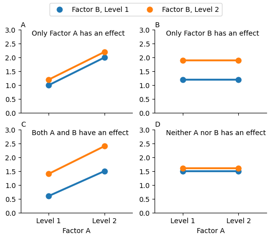
_images/8fc757cd7cb9a10f2e283e930de4ced7c4c25edb3489af7bdcbf81d4ed423bbd.png — Fig. 17.1 The four different outcomes for a 2 x 2 ANOVA when no interactions are present. In Panel A we see a main effect of Factor A, and no effect of Factor B. Panel B shows a main effect of Factor B but no effect of Factor A. Panel C shows main effects of both Factor A and Factor B. Finally, Panel D shows no effect of either factor.#

17.2. Balanced designs, main effects and interactions#

The four patterns of data shown in Fig. 17.1 are all quite realistic: there are a great many data sets that produce exactly those patterns. However, they are not the whole story, and the ANOVA model that we have been talking about up to this point is not sufficient to fully account for a table of group means. Why not? Well, so far we have the ability to talk about the idea that drugs can influence mood, and therapy can influence mood, but no way of talking about the possibility of an interaction between the two. An interaction between A and B is said to occur whenever the effect of Factor A is different, depending on which level of Factor B we’re talking about. Several examples of an interaction effect with the context of a 2 x 2 ANOVA are shown in Fig. 17.2. To give a more concrete example, suppose that the operation of Anxifree and Joyzepam is governed quite different physiological mechanisms, and one consequence of this is that while Joyzepam has more or less the same effect on mood regardless of whether one is in therapy, Anxifree is actually much more effective when administered in conjunction with CBT. The ANOVA that we developed in the previous section does not capture this idea. To get some idea of whether an interaction is actually happening here, it helps to plot the various group means.

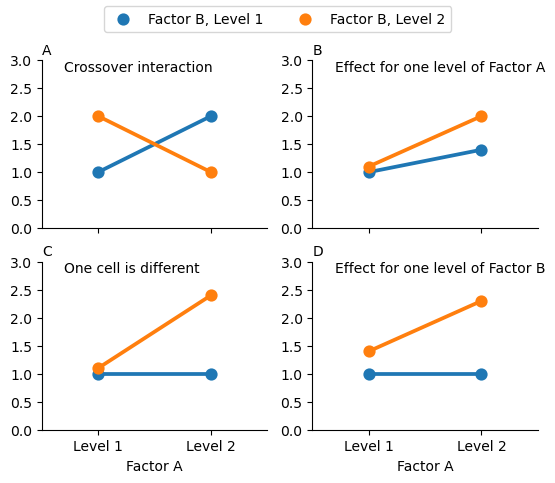
_images/75c83a691c2d04154f7eb4e81f8093ebe13b0ec5932ddce48ea98be004921005.png — Fig. 17.2 Qualitatively different interactions for a 2 x 2 ANOVA#

To give a more concrete example, suppose that the operation of Anxifree and Joyzepam is governed quite different physiological mechanisms, and one consequence of this is that while Joyzepam has more or less the same effect on mood regardless of whether one is in therapy, Anxifree is actually much more effective when administered in conjunction with CBT. The ANOVA that we developed in the previous section does not capture this idea. To get some idea of whether an interaction is actually happening here, it helps to plot the various group means. We can do this easily with seaborn:

sns.pointplot(data=df, x='drug', y='mood_gain', hue='therapy')
sns.despine()

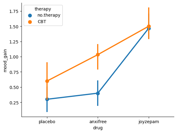
_images/b3ad66506061f50d80c39ef4063b2cac35789f94d8a17eac5cedbf8cd0d591a6.png

Our main concern relates to the fact that the two lines aren’t parallel. The effect of CBT (difference between solid line and dotted line) when the drug is Joyzepam (right side) appears to be near zero, even smaller than the effect of CBT when a placebo is used (left side). However, when Anxifree is administered, the effect of CBT is larger than the placebo (middle). Is this effect real, or is this just random variation due to chance? Our original ANOVA cannot answer this question, because we make no allowances for the idea that interactions even exist! In this section, we’ll fix this problem.

17.2.1. What exactly is an interaction effect?#

The key idea that we’re going to introduce in this section is that of an interaction effect. pingouin has already been calculating the for us, but to keep things simple, I have just ignored them. Now the time has come to look at that other line in the ANOVA table, the one that about “drug*therapy”.

Intuitively, the idea behind an interaction effect is fairly simple: it just means that the effect of Factor A is different, depending on which level of Factor B we’re talking about. But what does that actually mean in terms of our data? Fig. 17.2 depicts several different patterns that, although quite different to each other, would all count as an interaction effect. So it’s not entirely straightforward to translate this qualitative idea into something mathematical that a statistician can work with. As a consequence, the way that the idea of an interaction effect is formalised in terms of null and alternative hypotheses is slightly difficult, and I’m guessing that a lot of readers of this book probably won’t be all that interested. Even so, I’ll try to give the basic idea here.

To start with, we need to be a little more explicit about our main effects. Consider the main effect of Factor A (drug in our running example). We originally formulated this in terms of the null hypothesis that the two marginal means \(\mu_{r.}\) are all equal to each other. Obviously, if all of these are equal to each other, then they must also be equal to the grand mean \(\mu_{..}\) as well, right? So what we can do is define the effect of Factor A at level \(r\) to be equal to the difference between the marginal mean \(\mu_{r.}\) and the grand mean \(\mu_{..}\).

Let’s denote this effect by \(\alpha_r\), and note that

\[ \alpha_r = \mu_{r.} - \mu_{..} \]

Now, by definition all of the \(\alpha_r\) values must sum to zero, for the same reason that the average of the marginal means \(\mu_{r.}\) must be the grand mean \(\mu_{..}\). We can similarly define the effect of Factor B at level \(i\) to be the difference between the column marginal mean \(\mu_{.c}\) and the grand mean \(\mu_{..}\)

\[ \beta_c = \mu_{.c} - \mu_{..} \]

and once again, these \(\beta_c\) values must sum to zero. The reason that statisticians sometimes like to talk about the main effects in terms of these \(\alpha_r\) and \(\beta_c\) values is that it allows them to be precise about what it means to say that there is no interaction effect. If there is no interaction at all, then these \(\alpha_r\) and \(\beta_c\) values will perfectly describe the group means \(\mu_{rc}\). Specifically, it means that

\[ \mu_{rc} = \mu_{..} + \alpha_r + \beta_c \]

That is, there’s nothing special about the group means that you couldn’t predict perfectly by knowing all the marginal means. And that’s our null hypothesis, right there. The alternative hypothesis is that

\[ \mu_{rc} \neq \mu_{..} + \alpha_r + \beta_c \]

for at least one group \(rc\) in our table. However, statisticians often like to write this slightly differently. They’ll usually define the specific interaction associated with group \(rc\) to be some number, awkwardly referred to as \((\alpha\beta)_{rc}\), and then they will say that the alternative hypothesis is that

\[ \mu_{rc} = \mu_{..} + \alpha_r + \beta_c + (\alpha\beta)_{rc} \]

where \((\alpha\beta)_{rc}\) is non-zero for at least one group. This notation is kind of ugly to look at, but it is handy as we’ll see in the next section when discussing how to calculate the sum of squares.

17.2.2. Calculating sums of squares for the interaction#

How should we calculate the sum of squares for the interaction terms, SS\(_{A:B}\)?

Well, first off, it helps to notice how the previous section defined the interaction effect in terms of the extent to which the actual group means differ from what you’d expect by just looking at the marginal means. Of course, all of those formulas refer to population parameters rather than sample statistics, so we don’t actually know what they are. However, we can estimate them by using sample means in place of population means. So for Factor A, a good way to estimate the main effect at level \(r\) as the difference between the sample marginal mean \(\bar{Y}_{rc}\) and the sample grand mean \(\bar{Y}_{..}\). That is, we would use this as our estimate of the effect:

\[ \hat{\alpha}_r = \bar{Y}_{r.} - \bar{Y}_{..} \]

Similarly, our estimate of the main effect of Factor B at level \(c\) can be defined as follows:

\[ \hat{\beta}_c = \bar{Y}_{.c} - \bar{Y}_{..} \]

Now, if you go back to the formulas that I used to describe the SS values for the two main effects, you’ll notice that these effect terms are exactly the quantities that we were squaring and summing! So what’s the analog of this for interaction terms? The answer to this can be found by first rearranging the formula for the group means \(\mu_{rc}\) under the alternative hypothesis, so that we get this:

\[\begin{split} \begin{align} (\alpha \beta)_{rc} &= \mu_{rc} - \mu_{..} - \alpha_r - \beta_c \\ &= \mu_{rc} - \mu_{..} - (\mu_{r.} - \mu_{..}) - (\mu_{.c} - \mu_{..}) \\ & = \mu_{rc} - \mu_{r.} - \mu_{.c} + \mu_{..} \end{align} \end{split}\]

So, once again, if we substitute our sample statistics in place of the population means, we get the following as our estimate of the interaction effect for group \(rc\), which is

\[ \hat{(\alpha\beta)}_{rc} = \bar{Y}_{rc} - \bar{Y}_{r.} - \bar{Y}_{.c} + \bar{Y}_{..} \]

Now all we have to do is sum all of these estimates across all \(R\) levels of Factor A and all \(C\) levels of Factor B, and we obtain the following formula for the sum of squares associated with the interaction as a whole:

\[ \mbox{SS}_{A:B} = N \sum_{r=1}^R \sum_{c=1}^C \left( \bar{Y}_{rc} - \bar{Y}_{r.} - \bar{Y}_{.c} + \bar{Y}_{..} \right)^2 \]

where, we multiply by \(N\) because there are \(N\) observations in each of the groups, and we want our SS values to reflect the variation among observations accounted for by the interaction, not the variation among groups.

Now that we have a formula for calculating SS\(_{A:B}\), it’s important to recognise that the interaction term is part of the model (of course), so the total sum of squares associated with the model, SS\(_M\) is now equal to the sum of the three relevant SS values, \(\mbox{SS}_A + \mbox{SS}_B + \mbox{SS}_{A:B}\). The residual sum of squares \(\mbox{SS}_R\) is still defined as the leftover variation, namely \(\mbox{SS}_T - \mbox{SS}_M\), but now that we have the interaction term this becomes

\[ \mbox{SS}_R = \mbox{SS}_T - (\mbox{SS}_A + \mbox{SS}_B + \mbox{SS}_{A:B}) \]

As a consequence, the residual sum of squares SS\(_R\) will be smaller than in our original ANOVA that didn’t include interactions.

17.2.3. Degrees of freedom for the interaction#

Calculating the degrees of freedom for the interaction is, once again, slightly trickier than the corresponding calculation for the main effects. To start with, let’s think about the ANOVA model as a whole. Once we include interaction effects in the model, we’re allowing every single group to have a unique mean, \(\mu_{rc}\). For an \(R \times C\) factorial ANOVA, this means that there are \(R \times C\) quantities of interest in the model, and only the one constraint: all of the group means need to average out to the grand mean. So the model as a whole needs to have \((R\times C) - 1\) degrees of freedom. But the main effect of Factor A has \(R-1\) degrees of freedom, and the main effect of Factor B has \(C-1\) degrees of freedom. Which means that the degrees of freedom associated with the interaction is

\[\begin{split} \begin{align} df_{A:B} &= (R\times C - 1) - (R - 1) - (C -1 ) \\ &= RC - R - C + 1 \\ &= (R-1)(C-1) \end{align} \end{split}\]

which is just the product of the degrees of freedom associated with the row factor and the column factor.

What about the residual degrees of freedom? Because we’ve added interaction terms, which absorb some degrees of freedom, there are fewer residual degrees of freedom left over. Specifically, note that if the model with interaction has a total of \((R\times C) - 1\), and there are \(N\) observations in your data set that are constrained to satisfy 1 grand mean, your residual degrees of freedom now become \(N-(R \times C)-1+1\), or just \(N-(R \times C)\).

17.2.4. Interpreting the results#

Now we are in a position to understand all the rows in the ANOVA table that we saw earlier. Even if you skimmed lightly over the math in the previous section (and you would be forgiven if you did), hopefully you will now have some intuition for the differences between main effects and interaction effects. But what does it all mean, in the end?

Let’s quickly remind ourselves of the results of our factorial ANOVA:

model2 = pg.anova(dv='mood_gain', between=['drug', 'therapy'], data=df, detailed=True)
round(model2, 3)

	Source	SS	DF	MS	F	p-unc	np2
0	drug	3.453	2	1.727	31.714	0.000	0.841
1	therapy	0.467	1	0.467	8.582	0.013	0.417
2	drug * therapy	0.271	2	0.136	2.490	0.125	0.293
3	Residual	0.653	12	0.054	NaN	NaN	NaN

We can now see that while we do have a significant main effect of drug (\(F_{2,12} = 31.7, p <.001\)) and therapy type (\(F_{1,12} = 8.6, p=.013\)), there is no significant interaction between the two (\(F_{2,12} = 2.5, p = 0.125\)).

There’s a couple of very important things to consider when interpreting the results of factorial ANOVA. Firstly, there’s the same issue that we had with one-way ANOVA, which is that if you obtain a significant main effect of (say) drug, it doesn’t tell you anything about which drugs are different to one another. To find that out, you need to run additional analyses. We’ll talk about some analyses that you can run in the sections on contrasts and post-hoc tests. The same is true for interaction effects: knowing that there’s a significant interaction doesn’t tell you anything about what kind of interaction exists. Again, you’ll need to run additional analyses.

Secondly, there’s a very peculiar interpretation issue that arises when you obtain a significant interaction effect but no corresponding main effect. This happens sometimes. For instance, in the crossover interaction shown in Fig. 17.2), this is exactly what you’d find: in this case, neither of the main effects would be significant, but the interaction effect would be. This is a difficult situation to interpret, and people often get a bit confused about it. The general advice that statisticians like to give in this situation is that you shouldn’t pay much attention to the main effects when an interaction is present. The reason they say this is that, although the tests of the main effects are perfectly valid from a mathematical point of view, when there is a significant interaction effect, the main effects rarely test interesting hypotheses. Recall that the null hypothesis for a main effect is that the marginal means are equal to each other, and that a marginal mean is formed by averaging across several different groups. But if you have a significant interaction effect, then you know that the groups that comprise the marginal mean aren’t homogeneous, so it’s not really obvious why you would even care about those marginal means.

Here’s what I mean. Again, let’s stick with a clinical example. Suppose that we had a \(2 \times 2\) design comparing two different treatments for phobias (e.g., systematic desensitisation vs flooding), and two different anxiety reducing drugs (e.g., Anxifree vs Joyzepam). Now suppose what we found was that Anxifree had no effect when desensitisation was the treatment, and Joyzepam had no effect when flooding was the treatment. But both were pretty effective for the other treatment. This is a classic crossover interaction, and what we’d find when running the ANOVA is that there is no main effect of drug, but a significant interaction. Now, what does it actually mean to say that there’s no main effect? Well, it means that, if we average over the two different psychological treatments, then the average effect of Anxifree and Joyzepam is the same. But why would anyone care about that? When treating someone for phobias, it is never the case that a person can be treated using an “average” of flooding and desensitisation: that doesn’t make a lot of sense. You either get one or the other. For one treatment, one drug is effective; and for the other treatment, the other drug is effective. The interaction is the important thing; the main effect is kind of irrelevant.

This sort of thing happens a lot: the main effect are tests of marginal means, and when an interaction is present we often find ourselves not being terribly interested in marginal means, because they imply averaging over things that the interaction tells us shouldn’t be averaged! Of course, it’s not always the case that a main effect is meaningless when an interaction is present. Often you can get a big main effect and a very small interaction, in which case you can still say things like “drug A is generally more effective than drug B” (because there was a big effect of drug), but you’d need to modify it a bit by adding that “the difference in effectiveness was different for different psychological treatments”. In any case, the main point here is that whenever you get a significant interaction you should stop and think about what the main effect actually means in this context. Don’t automatically assume that the main effect is interesting.

17.2.5. Effect sizes#

The effect size calculations for a factorial ANOVA is pretty similar to those used in one way ANOVA. Specifically, we can use \(\eta^2\) (eta-squared) as simple way to measure how big the overall effect is for any particular term. As before, \(\eta^2\) is defined by dividing the sum of squares associated with that term by the total sum of squares. For instance, to determine the size of the main effect of Factor A, we would use the following formula

\[ \eta_A^2 = \frac{\mbox{SS}_{A}}{\mbox{SS}_{T}} \]

As before, this can be interpreted in much the same way as \(R^2\) in regression.[4] It tells you the proportion of variance in the outcome variable that can be accounted for by the main effect of Factor A. It is therefore a number that ranges from 0 (no effect at all) to 1 (accounts for all of the variability in the outcome). Moreover, the sum of all the \(\eta^2\) values, taken across all the terms in the model, will sum to the the total \(R^2\) for the ANOVA model. If, for instance, the ANOVA model fits perfectly (i.e., there is no within-groups variability at all!), the \(\eta^2\) values will sum to 1. Of course, that rarely if ever happens in real life.

However, when doing a factorial ANOVA, there is a second measure of effect size that people like to report, known as partial \(\eta^2\). This is the effect size measure that pingouin gives you by default. The idea behind partial \(\eta^2\) (which is sometimes denoted \(_p\eta^2\) or \(\eta^2_p\)) is that, when measuring the effect size for a particular term (say, the main effect of Factor A), you want to deliberately ignore the other effects in the model (e.g., the main effect of Factor B). That is, you would pretend that the effect of all these other terms is zero, and then calculate what the \(\eta^2\) value would have been. This is actually pretty easy to calculate. All you have to do is remove the sum of squares associated with the other terms from the denominator. In other words, if you want the partial \(\eta^2\) for the main effect of Factor A, the denominator is just the sum of the SS values for Factor A and the residuals:

\[ \mbox{partial } \eta^2_A = \frac{\mbox{SS}_{A}}{\mbox{SS}_{A} + \mbox{SS}_{R}} \]

This will always give you a larger number than \(\eta^2\), which the cynic in me suspects accounts for the popularity of partial \(\eta^2\). And once again you get a number between 0 and 1, where 0 represents no effect. However, it’s slightly trickier to interpret what a large partial \(\eta^2\) value means. In particular, you can’t actually compare the partial \(\eta^2\) values across terms! Suppose, for instance, there is no within-groups variability at all: if so, SS\(_R = 0\). What that means is that every term has a partial \(\eta^2\) value of 1. But that doesn’t mean that all terms in your model are equally important, or indeed that they are equally large. All it mean is that all terms in your model have effect sizes that are large relative to the residual variation. It is not comparable across terms.

To see what I mean by this, it’s useful to see a concrete example. We can get pingouin to report \(\eta^2\) instead of partial \(\eta^2\) by specifying this in the effsize argument when we run our ANOVA:

model2 = pg.anova(dv='mood_gain', 
                  between=['drug', 'therapy'], 
                  data=df, 
                  detailed=True, 
                  effsize='n2')
round(model2, 3)

	Source	SS	DF	MS	F	p-unc	n2
0	drug	3.453	2	1.727	31.714	0.000	0.713
1	therapy	0.467	1	0.467	8.582	0.013	0.096
2	drug * therapy	0.271	2	0.136	2.490	0.125	0.056
3	Residual	0.653	12	0.054	NaN	NaN	NaN

Looking at the \(\eta^2\) values first, we see that drug accounts for 71.3% of the variance (i.e. \(\eta^2 = 0.713\)) in mood_gain, whereas therapy only accounts for 9.6%. This leaves a total of 19.1% of the variation unaccounted for (i.e., the residuals constitute 19.1% of the variation in the outcome). Overall, this implies that we have a very large effect[5] of drug and a modest effect of therapy.

Now let’s look at the partial \(\eta^2\) values.

model2 = pg.anova(dv='mood_gain', 
                  between=['drug', 'therapy'], 
                  data=df, 
                  detailed=True, 
                  effsize='np2')
round(model2, 3)

	Source	SS	DF	MS	F	p-unc	np2
0	drug	3.453	2	1.727	31.714	0.000	0.841
1	therapy	0.467	1	0.467	8.582	0.013	0.417
2	drug * therapy	0.271	2	0.136	2.490	0.125	0.293
3	Residual	0.653	12	0.054	NaN	NaN	NaN

Because the effect of therapy isn’t all that large, controlling for it doesn’t make much of a difference, so the partial \(\eta^2\) for drug doesn’t increase very much, and we obtain a value of \(_p\eta^2 = 0.789\)). In contrast, because the effect of drug was very large, controlling for it makes a big difference, and so when we calculate the partial \(\eta^2\) for therapy you can see that it rises to \(_p\eta^2 = 0.336\). The question that we have to ask ourselves is, what do these partial \(\eta^2\) values actually mean? The way I generally interpret the partial \(\eta^2\) for the main effect of Factor A is to interpret it as a statement about a hypothetical experiment in which only Factor A was being varied. So, even though in this experiment we varied both A and B, we can easily imagine an experiment in which only Factor A was varied: the partial \(\eta^2\) statistic tells you how much of the variance in the outcome variable you would expect to see accounted for in that experiment. However, it should be noted that this interpretation – like many things associated with main effects – doesn’t make a lot of sense when there is a large and significant interaction effect.

17.3. Assumption checking#

As with one-way ANOVA, the key assumptions of factorial ANOVA are homogeneity of variance (all groups have the same standard deviation), normality of the residuals, and independence of the observations. The first two are things we can test for. The third is something that you need to assess yourself by asking if there are any special relationships between different observations. What about homogeneity of variance and normality of the residuals? As it turns out, these are pretty easy to check: it’s no different to the checks we did for a one-way ANOVA.

17.3.1. Levene test for homogeneity of variance#

To test whether the groups have the same variance, we can use the Levene test. The theory behind the Levene test has already been discussed, so I won’t discuss it again. The funny thing is, though, that while pacakges exist to perform a Levene test on factorial ANOVA models in e.g. R, I have not been able to find a package that does the same in Python. As of the date of writing this, I can only find examples of Levene’s tests being performed on one-way models in Python. However, as far as I can tell, all that one needs to do is to create a new column in the dataframe that represents the interaction of the two factors, and run the Levene’s test on that. This seems to give the same result as e.g. the R function levene() run on a two-way model with interactions, so I offer it here as my solution to this problem:

df['interaction'] = df['drug']+df['therapy']

pg.homoscedasticity(data=df, 
                    dv='mood_gain', 
                    group='interaction').round(5)

	W	pval	equal_var
levene	0.09545	0.99123	True

The fact that the Levene test is non-significant means that we can safely assume that the homogeneity of variance assumption is not violated.

17.3.2. Normality of residuals#

As with one-way ANOVA, we can test for the normality of residuals in a straightforward fashion. At the time of writing, pingouin doesn’t have a way to extract the residuals, so we will need to use statsmodels to run our ANOVA first, and then use the .resid method to extract the residuals from the model. Once we have done that, we can examine those residuals in a few different ways. It’s generally a good idea to examine them graphically, by drawing histograms (i.e., sns.histplot() function) and QQ plots (i.e., pg.qqplot() function. If you want a formal test for the normality of the residuals, then we can run the Shapiro-Wilk test (i.e., pg.normality()). If we wanted to check the residuals with respect to our two-way ANOVA (including interactions), we could first get the residuals using the following code:

import statsmodels.api as sm
from statsmodels.formula.api import ols

formula = 'mood_gain ~ drug + therapy + drug:therapy'

model = ols(formula, data=df).fit()
res = model.resid

As you can see from the formula variable above, in statsmodels we need to explicitly ask it to model the interactions for us, while pingouin does this automatically. We specify the interaction using :, so the interaction of drug and therapyis written as drug:therapy.

Now we can do our normality test:

pg.normality(res)

	W	pval	normal
0	0.928816	0.185093	True

I haven’t included the plots (you can draw them yourself if you want to see them), but you can see from the non-significance of the Shapiro-Wilk test that normality isn’t violated here.

17.4. The \(F\) test as a model comparison#

At this point, I want to talk in a little more detail about what the \(F\)-tests in an ANOVA are actually doing. In the context of ANOVA, I’ve been referring to the \(F\)-test as a way of testing whether a particular term in the model (e.g., main effect of Factor A) is significant. This interpretation is perfectly valid, but it’s not necessarily the most useful way to think about the test. In fact, it’s actually a fairly limiting way of thinking about what the \(F\)-test does. Consider the clinical trial data we’ve been working with in this chapter. Suppose I want to see if there are any effects of any kind that involve therapy. I’m not fussy: I don’t care if it’s a main effect or an interaction effect.[6] One thing I could do is look at the output for model2 earlier: in this model we did see a main effect of therapy (\(p=.013\)) but we did not see an interaction effect (\(p=.125\)). That’s kind of telling us what we want to know, but it’s not quite the same thing. What we really want is a single test that jointly checks the main effect of therapy and the interaction effect.

Given the way that I’ve been describing the ANOVA \(F\)-test up to this point, you’d be tempted to think that this isn’t possible. On the other hand, if you recall the chapter on regression, we were able to use \(F\)-tests to make comparisons between a wide variety of regression models. Perhaps something of that sort is possible with ANOVA? And of course, the answer here is yes. The thing that you really need to understand is that the \(F\)-test, as it is used in both ANOVA and regression, is really a comparison of two statistical models. One of these models is the full model (alternative hypothesis), and the other model is a simpler model that is missing one or more of the terms that the full model includes (null hypothesis). The null model cannot contain any terms that are not in the full model. In the example I gave above, the full model is model2, and it contains a main effect for therapy, a main effect for drug, and the drug by therapy interaction term. The null model would be model1 since it contains only the main effect of drug.

17.4.1. The \(F\) test comparing two models#

Let’s frame this in a slightly more abstract way. We’ll say that our full model can be written as a statsmodels formula that contains several different terms, say Y ~ A + B + C + D (remember that ~ here can be read as “predicted by”). Our null model only contains some subset of these terms, say Y ~ A + B. Some of these terms might be main effect terms, others might be interaction terms. It really doesn’t matter. The only thing that matters here is that we want to treat some of these terms as the “starting point” (i.e. the terms in the null model, A and B), and we want to see if including the other terms (i.e., C and D) leads to a significant improvement in model performance, over and above what could be achieved by a model that includes only A and B.

Is there a way of making this comparison directly?

To answer this, let’s go back to fundamentals. As we saw back when we learned about one-way ANOVA, the \(F\)-test is constructed from two kinds of quantity: sums of squares (SS) and degrees of freedom (df). These two things define a mean square value (MS = SS/df), and we obtain our \(F\) statistic by contrasting the MS value associated with “the thing we’re interested in” (the model) with the MS value associated with “everything else” (the residuals). What we want to do is figure out how to talk about the SS value that is associated with the difference between two models. It’s actually not all that hard to do.

Let’s start with the fundamental rule that we used throughout the chapter on regression:

\[ \mbox{SS}_{T} = \mbox{SS}_{M} + \mbox{SS}_{R} \]

That is, the total sums of squares (i.e., the overall variability of the outcome variable) can be decomposed into two parts: the variability associated with the model \(\mbox{SS}_{M}\), and the residual or leftover variability, \(\mbox{SS}_{R}\). However, it’s kind of useful to rearrange this equation slightly, and say that the SS value associated with a model is defined like this…

\[ \mbox{SS}_{M} = \mbox{SS}_{T} - \mbox{SS}_{R} \]

Now, in our scenario, we have two models: the null model (M0) and the full model (M1):

\[ \mbox{SS}_{M0} = \mbox{SS}_{T} - \mbox{SS}_{R0} \]

\[ \mbox{SS}_{M1} = \mbox{SS}_{T} - \mbox{SS}_{R1} \]

Next, let’s think about what it is we actually care about here. What we’re interested in is the difference between the full model and the null model. So, if we want to preserve the idea that what we’re doing is an “analysis of the variance” (ANOVA) in the outcome variable, what we should do is define the SS associated with the difference to be equal to the difference in the SS:

\[\begin{split} \begin{align} \mbox{SS}_{\Delta} &= \mbox{SS}_{M1} - \mbox{SS}_{M0}\\ &= (\mbox{SS}_{T} - \mbox{SS}_{R1}) - (\mbox{SS}_{T} - \mbox{SS}_{R0} ) \\ &= \mbox{SS}_{R0} - \mbox{SS}_{R1} \end{align} \end{split}\]

Now that we have our degrees of freedom, we can calculate mean squares and \(F\) values in the usual way. Specifically, we’re interested in the mean square for the difference between models, and the mean square for the residuals associated with the full model (M1), which are given by

\[\begin{split} \begin{align} \mbox{MS}_{\Delta} &= \frac{\mbox{SS}_{\Delta} }{ \mbox{df}_{\Delta} } \\ \mbox{MS}_{R1} &= \frac{ \mbox{SS}_{R1} }{ \mbox{df}_{R1} }\\ \end{align} \end{split}\]

Finally, taking the ratio of these two gives us our \(F\) statistic:

\[ F = \frac{\mbox{MS}_\Delta} {\mbox{MS}_{R1}} \]

17.4.2. Running the test in Python#

At this point, it may help to go back to our concrete example. The null model here is model1, which stipulates that there is a main effect of drug, but no other effects exist. We expressed this via the model formula mood_gain ~ drug. The alternative model here is model3, which stipulates that there is a main effect of drug, a main effect of therapy, and an interaction. This model corresponds to the formula mood_gain ~ drug + therapy + drug:therapy. The key thing here is that if we compare model1 to model3, we’re lumping the main effect of therapy and the interaction term together. Running this test in Python is straightforward: we just input both models to the anova_lm function from statsmodels, and it will run the exact F -test that I outlined above.

import pandas as pd
from statsmodels.formula.api import ols
from statsmodels.stats.anova import anova_lm

df = pd.read_csv("https://raw.githubusercontent.com/ethanweed/pythonbook/main/Data/clintrial.csv")

formula1 = 'mood_gain ~ drug'
formula2 = 'mood_gain ~ drug + therapy + drug:therapy'

model1 = ols(formula1, data=df).fit()
model2 = ols(formula2, data=df).fit()

anovaResults = anova_lm(model1, model2)
anovaResults

	df_resid	ssr	df_diff	ss_diff	F	Pr(>F)
0	15.0	1.391667	0.0	NaN	NaN	NaN
1	12.0	0.653333	3.0	0.738333	4.520408	0.024242

Let’s see if we can reproduce this \(F\)-test ourselves. Firstly, if you go back and look at the ANOVA tables that we printed out for model1 and model3 you can reassure yourself that the RSS values printed in this table really do correspond to the residual sum of squares associated with these two models. So let’s type them in as variables:

 ss_res_null = 1.391667
 ss_res_full = 0.653333

Now, following the procedure that I described above, we will say that the “between model” sum of squares, is the difference between these two residual sum of squares values. So, if we do the subtraction, we discover that the sum of squares associated with those terms that appear in the full model but not the null model is:

 ss_diff = ss_res_null - ss_res_full 
 ss_diff

0.7383339999999999

Right. Next, as always we need to convert these SS values into MS (mean square) values, which we do by dividing by the degrees of freedom. The degrees of freedom associated with the full-model residuals hasn’t changed from our original ANOVA for model2: it’s the total sample size \(N\), minus the total number of groups \(G\) that are relevant to the model. We have 18 people in the trial and 6 possible groups (i.e., 2 therapies \(\times\) 3 drugs), so the degrees of freedom here is 12. The degrees of freedom for the null model are calculated similarly. The only difference here is that there are only 3 relevant groups (i.e., 3 drugs), so the degrees of freedom here is 15. And, because the degrees of freedom associated with the difference is equal to the difference in the two degrees of freedom, we arrive at the conclusion that we have \(15-12 = 3\) degrees of freedom. Now that we know the degrees of freedom, we can calculate our MS values:

 ms_res = ss_res_full / 12
 ms_diff = ss_diff / 3 

Okay, now that we have our two MS values, we can divide one by the other, and obtain an \(F\)-statistic …

 F_stat = ms_diff / ms_res 
 F_stat

4.520414551231913

… and, just as we had hoped, this turns out to be nearly identical to the \(F\)-statistic that the anova_lm() function produced earlier.

17.5. ANOVA as a linear model#

One of the most important things to understand about ANOVA and regression is that they’re basically the same thing. On the surface of it, you wouldn’t think that this is true: after all, the way that I’ve described them so far suggests that ANOVA is primarily concerned with testing for group differences, and regression is primarily concerned with understanding the correlations between variables. And as far as it goes, that’s perfectly true. But when you look under the hood, so to speak, the underlying mechanics of ANOVA and regression are awfully similar. In fact, if you think about it, you’ve already seen evidence of this. ANOVA and regression both rely heavily on sums of squares (SS), both make use of \(F\) tests, and so on. Looking back, it’s hard to escape the feeling that the chapters on ANOVA and regression were a bit repetitive.

The reason for this is that ANOVA and regression are both kinds of linear models. In the case of regression, this is kind of obvious. The regression equation that we use to define the relationship between predictors and outcomes is the equation for a straight line, so it’s quite obviously a linear model. When we use e.g. a pingouin command like pg.linear_regression([predictor1, predictor2], outcome) what we’re really working with is the somewhat uglier linear model:

\[ Y_{p} = b_1 X_{1p} + b_2 X_{2p} + b_0 + \epsilon_{p} \]

where \(Y_p\) is the outcome value for the \(p\)-th observation (e.g., \(p\)-th person), \(X_{1p}\) is the value of the first predictor for the \(p\)-th observation, \(X_{2p}\) is the value of the second predictor for the \(p\)-th observation, the \(b_1\), \(b_2\) and \(b_0\) terms are our regression coefficients, and \(\epsilon_{p}\) is the \(p\)-th residual. If we ignore the residuals \(\epsilon_{p}\) and just focus on the regression line itself, we get the following formula:

\[ \hat{Y}_{p} = b_1 X_{1p} + b_2 X_{2p} + b_0 \]

where \(\hat{Y}_p\) is the value of \(Y\) that the regression line predicts for person \(p\), as opposed to the actually-observed value \(Y_p\). The thing that isn’t immediately obvious is that we can write ANOVA as a linear model as well. However, it’s actually pretty straightforward to do this. Let’s start with a really simple example: rewriting a \(2 \times 2\) factorial ANOVA as a linear model.

17.5.1. Some data#

To make things concrete, let’s suppose that our outcome variable is the grade that a student receives in my class, a ratio-scale variable corresponding to a mark from 0% to 100%. There are two predictor variables of interest: whether or not the student turned up to lectures (the attend variable), and whether or not the student actually read the textbook (the reading variable). We’ll say that attend = 1 if the student attended class, and attend = 0 if they did not. Similarly, we’ll say that reading = 1 if the student read the textbook, and reading = 0 if they did not.

Okay, so far that’s simple enough. The next thing we need to do is to wrap some maths around this (sorry!). For the purposes of this example, let \(Y_p\) denote the grade of the \(p\)-th student in the class. This is not quite the same notation that we used earlier in this chapter: previously, we’ve used the notation \(Y_{rci}\) to refer to the \(i\)-th person in the \(r\)-th group for predictor 1 (the row factor) and the \(c\)-th group for predictor 2 (the column factor). This extended notation was really handy for describing how the SS values are calculated, but it’s a pain in the current context, so I’ll switch notation here. Now, the \(Y_p\) notation is visually simpler than \(Y_{rci}\), but it has the shortcoming that it doesn’t actually keep track of the group memberships! That is, if I told you that \(Y_{0,0,3} = 35\), you’d immediately know that we’re talking about a student (the 3rd such student, in fact) who didn’t attend the lectures (i.e., attend = 0) and didn’t read the textbook (i.e. reading = 0), and who ended up failing the class (grade = 35). But if I tell you that \(Y_p = 35\) all you know is that the \(p\)-th student didn’t get a good grade. We’ve lost some key information here. Of course, it doesn’t take a lot of thought to figure out how to fix this: what we’ll do instead is introduce two new variables \(X_{1p}\) and \(X_{2p}\) that keep track of this information. In the case of our hypothetical student, we know that \(X_{1p} = 0\) (i.e., attend = 0) and \(X_{2p} = 0\) (i.e., reading = 0). So the data might look like this:

person \(p\)	grade \(Y_p\)	attendance \(X_{1p}\)	reading \(X_{2p}\)
1	90	1	1
2	87	1	1
3	75	0	1
4	60	1	0
5	35	0	0
6	50	0	0
7	65	1	0
8	70	0	1

This isn’t anything particularly special, of course: it’s exactly the format in which we expect to see our data! In other words, if your data have been stored as a pandas data frame, then you’re probably expecting to see something that looks like the rtfm1 data frame:

rtfm1 = pd.read_csv('https://raw.githubusercontent.com/ethanweed/pythonbook/main/Data/rtfm1.csv')
rtfm1

	grade	attend	reading
0	90	1	1
1	87	1	1
2	75	0	1
3	60	1	0
4	35	0	0
5	50	0	0
6	65	1	0
7	70	0	1

Well, sort of. I suspect that a few readers are probably frowning a little at this point. Earlier on in the book (for example back when we talked about the McNemar test),we have typically represented nominal scale variables such as attend and reading as text, rather than encoding them as numeric variables. The rtfm1 data frame doesn’t do this, but the rtfm2 data frame does, and so you might instead be expecting to see data like this:

rtfm2 = pd.read_csv('https://raw.githubusercontent.com/ethanweed/pythonbook/main/Data/rtfm2.csv')
rtfm2

	grade	attend	reading
0	90	yes	yes
1	87	yes	yes
2	75	no	yes
3	60	yes	no
4	35	no	no
5	50	no	no
6	65	yes	no
7	70	no	yes

However, for the purposes of this section it’s important that we be able to switch back and forth between these two different ways of thinking about the data. After all, our goal in this section is to look at some of the mathematics that underpins ANOVA, and if we want to do that we need to be able to see the numerical representation of the data (in rtfm1) as well as the more meaningful factor representation (in rtfm2). We will return to this problem however, because it is not irrelevant which numbers we use to represent our categories. For now, however, we are on safe ground with our 0’s and 1’s, so let’s proceed and confirm that this data set corresponds to a balanced design:

pd.crosstab(rtfm2['attend'], rtfm2['reading'])

reading	no	yes
attend
no	2	2
yes	2	2

For each possible combination of the attend and reading variables, we have exactly two students. If we’re interested in calculating the mean grade for each of these cells,

rtfm_agg = rtfm2.groupby(['attend', 'reading']).mean()
rtfm_agg

		grade
attend	reading
no	no	42.5
no	yes	72.5
yes	no	62.5
yes	yes	88.5

Looking at this table, one gets the strong impression that reading the text and attending the class both matter a lot.

17.5.2. ANOVA with binary factors as a regression model#

Okay, let’s get back to talking about the mathematics. We now have our data expressed in terms of three numeric variables: the continuous variable \(Y\), and the two binary variables \(X_1\) and \(X_2\). What I want to you to recognise is that our 2\(\times\)2 factorial ANOVA is exactly equivalent to the regression model

\[ Y_{p} = b_1 X_{1p} + b_2 X_{2p} + b_0 + \epsilon_p \]

This is, of course, the exact same equation that I used earlier to describe a two-predictor regression model! The only difference is that \(X_1\) and \(X_2\) are now binary variables (i.e., values can only be 0 or 1), whereas in a regression analysis we expect that \(X_1\) and \(X_2\) will be continuous. There’s a couple of ways I could try to convince you of this. One possibility would be to do a lengthy mathematical exercise, proving that the two are identical. However, I’m going to go out on a limb and guess that most of the readership of this book will find that to be annoying rather than helpful. Instead, I’ll explain the basic ideas, and then rely on Python to show that that ANOVA analyses and regression analyses aren’t just similar, they’re identical for all intents and purposes. Let’s start by running this as an ANOVA.

Now, you may remember that back when we ran one-way ANOVAs, I said I thought the statsmodels package was great, but I also gushed about how we could use good old pingouin too. For this example, I am going to use statsmodels. I’ll explain why in a bit, but first let’s run our ANOVA:

import statsmodels.api as sm
from statsmodels.formula.api import ols

# Here we define our model.

model = ols('grade ~ attend + reading', data=rtfm1).fit()
sm.stats.anova_lm(model, typ=2).round(3)

	sum_sq	df	F	PR(>F)
attend	648.0	1.0	21.600	0.006
reading	1568.0	1.0	52.267	0.001
Residual	150.0	5.0	NaN	NaN

So, by reading the key numbers off the ANOVA table and the table of means that we presented earlier, we can see that the students obtained a higher grade if they attended class \((F_{1,5} = 26.1, p = .0056)\) and if they read the textbook \((F_{1,5} = 52.3, p = .0008)\).

Now let’s think about the same analysis from a linear regression perspective. In the rtfm1 data set, we have encoded attend and reading as if they were numeric predictors. In this case, this is perfectly acceptable. There really is a sense in which a student who turns up to class (i.e. attend = 1) has in fact done “more attendance” than a student who does not (i.e. attend = 0). So it’s not at all unreasonable to include it as a predictor in a regression model. It’s a little unusual, because the predictor only takes on two possible values, but it doesn’t violate any of the assumptions of linear regression. And it’s easy to interpret. If the regression coefficient for attend is greater than 0, it means that students that attend lectures get higher grades; if it’s less than zero, then students attending lectures get lower grades. The same is true for our reading variable.

Wait a second… why is this true? It’s something that is intuitively obvious to everyone who has taken a few stats classes and is comfortable with the maths, but it isn’t clear to everyone else at first pass. To see why this is true, it helps to look closely at a few specific students. Let’s start by considering the 6th and 7th students in our data set (i.e. \(p=6\) and \(p=7\)). Neither one has read the textbook, so in both cases we can set reading = 0. Or, to say the same thing in our mathematical notation, we observe \(X_{2,6} = 0\) and \(X_{2,7} = 0\). However, student number 7 did turn up to lectures (i.e., attend = 1, \(X_{1,7} = 1\)) whereas student number 6 did not (i.e., attend = 0, \(X_{1,6} = 0\)). Now let’s look at what happens when we insert these numbers into the general formula for our regression line. For student number 6, the regression predicts that

\[\begin{split} \begin{array} \hat{Y}_{6} &=& b_1 X_{1,6} + b_2 X_{2,6} + b_0 \\ &=& (b_1 \times 0) + ( b_2 \times 0) + b_0 \\ &=& b_0 \end{array} \end{split}\]

So we’re expecting that this student will obtain a grade corresponding to the value of the intercept term \(b_0\). What about student 7? This time, when we insert the numbers into the formula for the regression line, we obtain the following:

\[\begin{split} \begin{array} \hat{Y}_{7} &=& b_1 X_{1,7} + b_2 X_{2,7} + b_0 \\ &=& (b_1 \times 1) + ( b_2 \times 0) + b_0 \\ &=& b_1 + b_0 \end{array} \end{split}\]

Because this student attended class, the predicted grade is equal to the intercept term \(b_0\) plus the coefficient associated with the attend variable, \(b_1\). So, if \(b_1\) is greater than zero, we’re expecting that the students who turn up to lectures will get higher grades than those students who don’t. If this coefficient is negative, we’re expecting the opposite: students who turn up at class end up performing much worse. In fact, we can push this a little bit further. What about student number 1, who turned up to class (\(X_{1,1} = 1\)) and read the textbook (\(X_{2,1} = 1\))? If we plug these numbers into the regression, we get

\[\begin{split} \begin{array} \hat{Y}_{1} &=& b_1 X_{1,1} + b_2 X_{2,1} + b_0 \\ &=& (b_1 \times 1) + ( b_2 \times 1) + b_0 \\ &=& b_1 + b_2 + b_0 \end{array} \end{split}\]

So if we assume that attending class helps you get a good grade (i.e., \(b_1 > 0\)) and if we assume that reading the textbook also helps you get a good grade (i.e., \(b_2 >0\)), then our expectation is that student 1 will get a grade that that is higher than student 6 and student 7.

And at this point, you won’t be at all suprised to learn that the regression model predicts that student 3, who read the book but didn’t attend lectures, will obtain a grade of \(b_2 + b_0\). I won’t bore you with yet another regression formula. Instead, what I’ll do is show you the following table of expected grades:

		read textbook?
		no	yes
attended?	no	\(b_0\)	\(b_0 + b_2\)
	yes	\(b_0 + b_1\)”	\(b_0 + b_1 + b_2\)

As you can see, the intercept term \(b_0\) acts like a kind of “baseline” grade that you would expect from those students who don’t take the time to attend class or read the textbook. Similarly, \(b_1\) represents the boost that you’re expected to get if you come to class, and \(b_2\) represents the boost that comes from reading the textbook. In fact, if this were an ANOVA you might very well want to characterise \(b_1\) as the main effect of attendance, and \(b_2\) as the main effect of reading! In fact, for a simple \(2 \times 2\) ANOVA that’s exactly how it plays out.

Okay, now that we’re really starting to see why ANOVA and regression are basically the same thing, let’s actually run our regression using a regression function to convince ourselves that this is really true. And this brings us to the first reason for using statsmodels for this example rather than pingouin. If you look back at the code we used to run our ANOVA, you will see that it was this:

model = ols('grade ~ attend + reading', data=rtfm2).fit() `sm.stats.anova_lm(model, typ=2).round(4)```

That is to say, we already ran a regression! Our variable model literally is a linear regression, and all we did with sm.stats.anova_lm was dress up the results in an ANOVA costume[7]

Let’s take a closer look at the output of that regression we did. statsmodels spits out a lot of information, but I just want to zoom in on the part that is relevant for us now, which can be found like this:

model.summary().tables[1]

/Users/ethan/opt/miniconda3/envs/pythonbook3/lib/python3.11/site-packages/scipy/stats/_stats_py.py:1736: UserWarning: kurtosistest only valid for n>=20 ... continuing anyway, n=8
  warnings.warn("kurtosistest only valid for n>=20 ... continuing "

	coef	std err	t	P>\|t\|	[0.025	0.975]
Intercept	43.5000	3.354	12.969	0.000	34.878	52.122
attend	18.0000	3.873	4.648	0.006	8.044	27.956
reading	28.0000	3.873	7.230	0.001	18.044	37.956

There’s a few interesting things to note here. First, notice that the intercept term is 43.5, which is close to the “group” mean of 42.5 observed for those two students who didn’t read the text or attend class. Second, notice that we have the regression coefficient of \(b_1 = 18.0\) for the attendance variable, suggesting that those students that attended class scored 18% higher than those who didn’t. So our expectation would be that those students who turned up to class but didn’t read the textbook would obtain a grade of \(b_0 + b_1\), which is equal to \(43.5 + 18.0 = 61.5\). Again, this is similar to the observed group mean of 62.5. You can verify for yourself that the same thing happens when we look at the students that read the textbook.

Actually, we can push a little further in establishing the equivalence of our ANOVA and our regression. Look at the \(p\)-values associated with the attend variable and the reading variable in the regression output. They’re identical to the ones we encountered earlier when running the ANOVA. This might seem a little surprising, since the test used when running our regression model calculates a \(t\)-statistic and the ANOVA calculates an \(F\)-statistic. However, if you can remember all the way back to the chapter on probability, I mentioned that there’s a relationship between the \(t\)-distribution and the \(F\)-distribution: if you have some quantity that is distributed according to a \(t\)-distribution with \(k\) degrees of freedom and you square it, then this new squared quantity follows an \(F\)-distribution whose degrees of freedom are 1 and \(k\). We can check this with respect to the \(t\) statistics in our regression model. For the attend variable we get a \(t\) value of 4.648. If we square this number we end up with 21.604, which is identical to the corresponding \(F\) statistic in our ANOVA. I love it when a plan comes together.

I mentioned there was a second reason I didn’t use pingouin for this example. This is because as far as I can tell, when performing an ANOVA pingouin always calculates not only the main effects, but also the interaction, thus giving slightly different results. In order to keep things simple (and maintain parity with LSR, I decided to go with statsmodels and not specify any interactions. Just to be sure though, let’s run the ANOVA with pingouin, and then run the regression in statsmodels with a little ANOVA dressing on top, and confirm that we get the same result:

pg.anova(dv='grade', between=['attend', 'reading'], data=rtfm1).round(3)

	Source	SS	DF	MS	F	p-unc	np2
0	attend	648.0	1	648.0	18.254	0.013	0.820
1	reading	1568.0	1	1568.0	44.169	0.003	0.917
2	attend * reading	8.0	1	8.0	0.225	0.660	0.053
3	Residual	142.0	4	35.5	NaN	NaN	NaN

model = ols('grade ~ attend + reading + attend:reading', data=rtfm1).fit()
sm.stats.anova_lm(model, typ=2).round(3)

	sum_sq	df	F	PR(>F)
attend	648.0	1.0	18.254	0.013
reading	1568.0	1.0	44.169	0.003
attend:reading	8.0	1.0	0.225	0.660
Residual	142.0	4.0	NaN	NaN

Yup. Same thing.

(changingbaseline) =

17.5.3. Changing the baseline category#

At this point, you’re probably convinced that the ANOVA and the regression are actually identical to each other. So there’s one last thing I should show you. What happens if I use the data from rtfm2 to run the regression? In rtfm2, we coded the attend and reading variables as text rather than as numeric variables. Does this matter? In this case, it turns out that it doesn’t. The only differences are superficial:

# With factors encoded numerically
model = ols('grade ~ attend + reading', data=rtfm1).fit()
model.summary().tables[1]

/Users/ethan/opt/miniconda3/envs/pythonbook3/lib/python3.11/site-packages/scipy/stats/_stats_py.py:1736: UserWarning: kurtosistest only valid for n>=20 ... continuing anyway, n=8
  warnings.warn("kurtosistest only valid for n>=20 ... continuing "

	coef	std err	t	P>\|t\|	[0.025	0.975]
Intercept	43.5000	3.354	12.969	0.000	34.878	52.122
attend	18.0000	3.873	4.648	0.006	8.044	27.956
reading	28.0000	3.873	7.230	0.001	18.044	37.956

# With factors encoded as text
model = ols('grade ~ attend + reading', data=rtfm2).fit()
model.summary().tables[1]

/Users/ethan/opt/miniconda3/envs/pythonbook3/lib/python3.11/site-packages/scipy/stats/_stats_py.py:1736: UserWarning: kurtosistest only valid for n>=20 ... continuing anyway, n=8
  warnings.warn("kurtosistest only valid for n>=20 ... continuing "

	coef	std err	t	P>\|t\|	[0.025	0.975]
Intercept	43.5000	3.354	12.969	0.000	34.878	52.122
attend[T.yes]	18.0000	3.873	4.648	0.006	8.044	27.956
reading[T.yes]	28.0000	3.873	7.230	0.001	18.044	37.956

The only thing that is different is that statsmodels labels the two variables differently: the output now refers to attend[T.yes] and reading[T.yes]. You can probably guess what this means. When statsmodels refers to reading[T.yes] it’s trying to indicate that it is assuming that “yes = 1” and “no = 0”. This is important for two reasons, one having to do with textually-encoded categories, and one having to do with numerically-encoded categories.

Let’s take the textually-encoded categories first. Suppose we wanted to say that “yes = 0” and “no = 1”. We could still run this as a regression model, but now all of our coefficients will go in the opposite direction, because the effect of reading[T.no] would be referring to the consequences of not reading the textbook.

We can do this in statsmodels by using the Treatment syntax, and manually specifiying the reference variable, like so:

model = ols('grade ~ C(attend) + C(reading, Treatment(reference="yes"))', data=rtfm2).fit()
model.summary().tables[1]

/Users/ethan/opt/miniconda3/envs/pythonbook3/lib/python3.11/site-packages/scipy/stats/_stats_py.py:1736: UserWarning: kurtosistest only valid for n>=20 ... continuing anyway, n=8
  warnings.warn("kurtosistest only valid for n>=20 ... continuing "

	coef	std err	t	P>\|t\|	[0.025	0.975]
Intercept	71.5000	3.354	21.317	0.000	62.878	80.122
C(attend)[T.yes]	18.0000	3.873	4.648	0.006	8.044	27.956
C(reading, Treatment(reference="yes"))[T.no]	-28.0000	3.873	-7.230	0.001	-37.956	-18.044

If we compare these results with the results using the default reference above, we see that the overall result has not changed (e.g. the p-value for “reading” is still 0.001, but the direction of the result is the opposite.

So how does statsmodels choose the reference level, if we do not specify it manually? The answer is simple, if a little arbitrary: it just goes by alphabetical order. Yup. N comes before Y in the alphabet, so “No” is picked as the reference level.

As it happens, this corresponds nicely with our numeric encoding, in which “No” was coded as 0, and “Yes” as 1, and 0 comes before 1 in the number line, but this will not necessarily be the case, so we need to stay alert, especially when using text to encode our levels. In the (admittedly unlikely) event that we had labelled our data “affirmative” and “negative” instead of “yes” and “no”, the direction of our results would be reversed, and we might not even notice!

rtfm3 = rtfm1
rtfm3['attend'] =[4,4,1,4,1,1,4,1]
rtfm3

	grade	attend	reading
0	90	4	1
1	87	4	1
2	75	1	1
3	60	4	0
4	35	1	0
5	50	1	0
6	65	4	0
7	70	1	1

model = ols('grade ~ attend + reading', data=rtfm3).fit()
model.summary().tables[1]

/Users/ethan/opt/miniconda3/envs/pythonbook3/lib/python3.11/site-packages/scipy/stats/_stats_py.py:1736: UserWarning: kurtosistest only valid for n>=20 ... continuing anyway, n=8
  warnings.warn("kurtosistest only valid for n>=20 ... continuing "

	coef	std err	t	P>\|t\|	[0.025	0.975]
Intercept	37.5000	4.233	8.859	0.000	26.619	48.381
attend	6.0000	1.291	4.648	0.006	2.681	9.319
reading	28.0000	3.873	7.230	0.001	18.044	37.956

17.5.4. How to encode non binary factors as contrasts#

At this point, I’ve shown you how we can view a \(2\times 2\) ANOVA into a linear model. And it’s pretty easy to see how this generalises to a \(2 \times 2 \times 2\) ANOVA or a \(2 \times 2 \times 2 \times 2\) ANOVA… it’s the same thing, really: you just add a new binary variable for each of your factors. Where it begins to get trickier is when we consider factors that have more than two levels. Consider, for instance, the \(3 \times 2\) ANOVA that we ran earlier in this chapter using the clin.trial data. How can we convert the three-level drug factor into a numerical form that is appropriate for a regression?

The answer to this question is pretty simple, actually. All we have to do is realise that a three-level factor can be redescribed as two binary variables. Suppose, for instance, I were to create a new binary variable called druganxifree. Whenever the drug variable is equal to "anxifree" we set druganxifree = 1. Otherwise, we set druganxifree = 0. This variable sets up a contrast, in this case between anxifree and the other two drugs. By itself, of course, the druganxifree contrast isn’t enough to fully capture all of the information in our drug variable. We need a second contrast, one that allows us to distinguish between joyzepam and the placebo. To do this, we can create a second binary contrast, called drugjoyzepam, which equals 1 if the drug is joyzepam, and 0 if it is not. Taken together, these two contrasts allows us to perfectly discriminate between all three possible drugs. The table below illustrates this:

	grade	attend	reading
0	90	yes	yes
1	87	yes	yes
2	75	no	yes
3	60	yes	no
4	35	no	no
5	50	no	no
6	65	yes	no
7	70	no	yes

	grade	attend	reading
0	90	yes	yes
1	87	yes	yes
2	75	no	yes
3	60	yes	no
4	35	no	no
5	50	no	no
6	65	yes	no
7	70	no	yes

Factorial ANOVA

Contents

17. Factorial ANOVA#

17.1. Balanced designs, main effects#

17.1.1. What hypotheses are we testing?#

17.1.2. Running the analysis in Python#

17.1.3. What are our degrees of freedom?#

17.1.4. Factorial ANOVA versus one-way ANOVAs#

17.1.5. What kinds of outcomes does this analysis capture?#

17.2. Balanced designs, main effects and interactions#

17.2.1. What exactly is an interaction effect?#

17.2.2. Calculating sums of squares for the interaction#

17.2.3. Degrees of freedom for the interaction#

17.2.4. Interpreting the results#

17.2.5. Effect sizes#

17.3. Assumption checking#

17.3.1. Levene test for homogeneity of variance#

17.3.2. Normality of residuals#

17.4. The \(F\) test as a model comparison#

17.4.1. The \(F\) test comparing two models#

17.4.2. Running the test in Python#

17.5. ANOVA as a linear model#

17.5.1. Some data#

17.5.2. ANOVA with binary factors as a regression model#

17.5.3. Changing the baseline category#

17.5.4. How to encode non binary factors as contrasts#

17.5.5. The equivalence between ANOVA and regression for non-binary factors#

17.5.6. Degrees of freedom as parameter counting!#

17.5.7. A postscript#

17.6. Different ways to specify contrasts#

17.6.1. Treatment contrasts#

17.6.2. Helmert contrasts#

17.6.3. Sum to zero contrasts#

17.6.4. Setting contrasts#

17.7. Post hoc tests#

17.8. Unbalanced designs#

17.8.1. The coffee data#

17.8.2. “Standard ANOVA” does not exist for unbalanced designs#

17.8.3. Type I sum of squares#

17.8.4. Type III sum of squares#

17.8.5. Type II sum of squares#

17.8.6. Effect sizes (and non-additive sums of squares)#

17.9. Summary#

	grade	attend	reading
0	90	yes	yes
1	87	yes	yes
2	75	no	yes
3	60	yes	no
4	35	no	no
5	50	no	no
6	65	yes	no
7	70	no	yes